Bidomain Model

This is the third writeup where I'll be documenting my research with Dr. Joyce Lin. If you want to read my introductory article regarding the research series, you can check it out here.

Introduction

The bidomain model is a mathematical model like the cable equation model which attempts to define the propagation of action potentials through the heart. The model itself was proposed by Tung and Geselowitz in the late 1970s. [1]

The model presents a more realistic approach when compared to the cable equation model due to its consideration of both the intracellular and extracellular spaces. It can also be considered as a higher order version of the cable equation.

A thing to keep note of is that this model is a first order approximation to a full detailed model thus the realism gets watered down when compared to newer models (like the microdomain model) due to its homogenization of the fine micro-structure that exists within both the intracellular and extracellular spaces.

Equation

The governing equations are as follows:

For intracellular spaces:

\chi \left( C_m \frac{\partial V}{\partial t} + I_{ion} \right) = \nabla \cdot (\sigma_i \nabla V_i)

For extracellular spaces:

\chi \left( C_m \frac{\partial V}{\partial t} + I_{ion} \right) = -\nabla \cdot (\sigma_e \nabla V_e)

Here,

$\chi$ is the membrane surface-to-volume ratio, needed to convert the transmembrane current per unit area into transmembrane current per unit volume.
$C_m$ represents the membrane capacitance.
$\frac{\partial V}{\partial t}$ represents the small minute change in potential across time.
$I_{ion}$ represents the ionic current.
For our simulation, we use the Hodgkin-Huxley Equations.
$\nabla$ represents the gradient/laplacian
$\sigma_i$ and $\sigma_e$ represent the conductivity tensors for the intracellular and extracellular spaces respectively.

Bidomain schema diagram
Representation of intracellular and extracellular space in bidomain model [2]

Assumptions required for the bidomain model

\nabla \cdot i_T = 0 \quad \text{where} \quad i_T = i_i + i_e

Another assumption here is that the total current is conserved. Homogenizing the fine microstructure of both the intracellular and extracellular spaces will not bring forward adverse effects in regards to the accuracy of the model.

The membrane parameter $C_m$ is constant and does not depend on the transmembrane potential.

Simulation

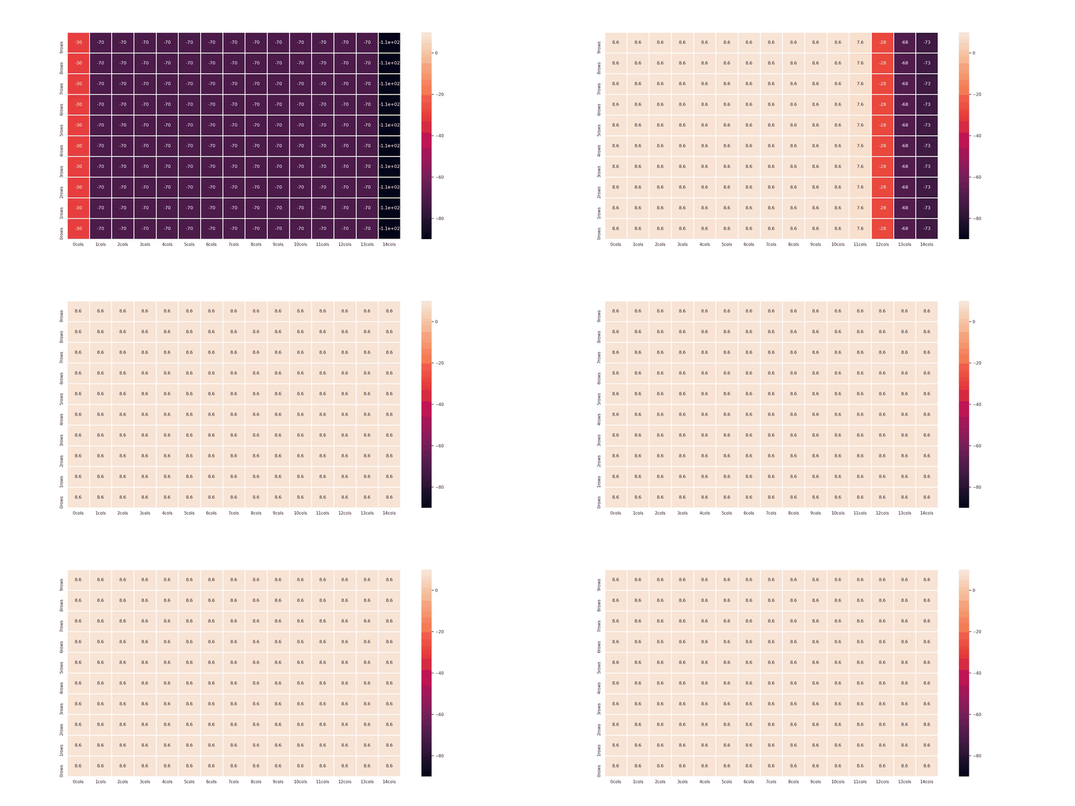
Considering all of the above assumptions, I was able to model the behavior of the action potential as it traverses through the cardiac tissue. The simulation below is an animation of multiple snapshots in time (in seconds) of the transmembrane potential (in mV) vs points space of the tissue (in cm). The simulation itself was coded up using Python and related libraries (Numpy, Pandas, Matplotlib, seaborn). To view the code behind the simulation, click here.

Here the tissue starts out with a resting potential of -70 mV and is given a stimulus by holding the opposite ends of the tissue at 40mV and -40mV respectively to create a potential difference. This stimulus is given for only 5 time steps (1 time step = ~0.01 sec). With this short stimulus, the progression of the action potential begins.

Another important note is that each frame of this simulation is a snapshot for every 600 time steps, thus giving us a sped up progression of the action potential.

The entire source code is available here.

Citations

[1] Keener, Sneyd, and Sneyd, James. Mathematical Physiology: I: Cellular Physiology. 2nd Ed. 2009. ed. New York, NY: Springer New York : Imprint: Springer, 2009. Interdisciplinary Applied Mathematics, 8/1. Web.

[2] Ibrahim, A. , Adediji, A. and Olufemi, D. (2013) Dynamical modelling of cardiac electrical activity using bidomain approach: The effects of variation of ionic model parameters. Journal of Biomedical Science and Engineering, 6, 598-608. doi: 10.4236/jbise.2013.66076.

By Srirag Vuppala

Jun 1st 2021